
Turtles “run” at 10 centimeters per second, while peregrine falcons might exceed 300 km/h when hunting pigeons. We often hear expressions like these, and we know they refer to how fast beings or objects are. But what does “being fast” or “being slow” really mean?
Velocity is a physical quantity that relates a body’s changes in position, or its movement, to the time it takes it to perform said change. It is one of the most common variables in cinematics —the branch of mechanics that studies movement—, and a very useful one in everyday life.
Let’s learn what velocity is really about, what are its types and how to calculate them.
How to calculate velocity
To calculate an object’s velocity follow these steps:
- Calculate the body’s displacement vector. Its magnitude, x, equals the difference between the final and the initial positions, measured with respect to an external reference system.
- Measure the time frame, t, within which the object moved from the initial to the final position.
- Use the following equation to calculate the object’s average velocity:

The average velocity direction equals that of the displacement vector.
What is the average velocity?
Velocity expresses how fast bodies move. But, what do we mean exactly by that? Movement is the change in a body’s position, and it has two main characteristics: its displacement and its trajectory. The first one refers to the net change in a body’s location with respect to a fixed reference point outside of it, while the second one refers to the pathway it follows when moving. Let’s try and understand this with an example:
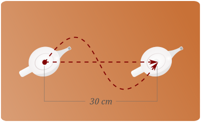
Imagine you put a teapot on a table. A friend of yours wants to have some tea, so you push the teapot across the surface 30 cm to the right in a straight line. If we fix a reference point right at the initial spot and measure the length to the teapot’s final position, which equals 30 cm, we would have measured the magnitude of its displacement.
On the other hand, if you had moved the teapot not in a straight line but in different directions before leaving it at the same final position as before, its displacement would have been the same, namely 30 cm, but its trajectory would have been definitely longer. The following image illustrates this. The dotted lines represent two possible trajectories when moving the teapot.
If an object moves and then returns to its initial position, its displacement would be zero, but its trajectory would be greater than zero. Go ahead and read our article on how to calculate displacement to learn more about this important concept.
Back to velocity! When objects move they change their position with respect to an external point of reference. By external we mean one that is not located within the moving object. In our previous example, if we were to measure the teapot’s position with respect to the teapot itself, the result would always be zero, since the reference would be moving with the object of interest.
Now we know when an object moves. So, the next question to understand the concept of velocity is how fast does it occur? All of the changes of an object’s position occur within a given amount of time. This means, no movement can occur instantaneously, since that would imply the object covered a certain distance in zero seconds. This is, according to classical physics, simply impossible.
Now, an object can experience the same amount of movement within different time periods. In our teapot example, you could probably slide it 30 cm across the table in just a few seconds. Nevertheless, you could have done it in twice the time or even in a shorter time frame. So we can think of a relationship between an object’s movement and the time it takes to cover the travelled distance.
That relation is the object’s velocity. More precisely, its speed. Go ahead and read the section titled Difference between velocity and speed to learn more about this. Velocity is then defined as the rate at which movement occurs.
On the one hand, movement can be represented by its displacement, which is a vector whose magnitude is the difference between the final and the initial positions of the object measured with respect to an external point of reference. This is usually represented as x. The vector’s direction simply points from the starting to the finishing points of the object’s trajectory.
On the other hand, a time frame can be measured as the final time minus the initial time, which is usually written as t. Since we are using the object’s displacement to define its velocity, the result is called its average velocity. This is because the resulting vector does not represent how fast the object is moving at a specific point of time, but how fast the total displacement was. The average velocity is then defined as shown in equation 1, and it has units of length over time (m/s, km/h, miles/h, etc.).
Keep in mind that the symbol (a capitalized greek delta) represents the change in a variable between an initial and a final state. It is defined as the final value minus the initial value.
Since the object’s displacement is a vector, its average velocity must also be a vector according to equation 1. In this case, its direction equals that of the object’s displacement.
So, if the movement takes place on a straight line, along which we can conveniently set a reference axis, the object’s velocity has that same direction. Things get more complex once two- or three-dimensional movement is studied, since calculating the displacement vector’s direction requires the consideration of displacement components along two or three individual axes, respectively. See our article on displacement to learn more about this.
What is the instantaneous velocity?
Velocity is a function of time. This means it can change as time passes. Imagine you take a car and drive from your house to another town nearby. Whether to wait at a red light or to allow someone to cross the street, you will probably have to slow down or even stop completely at some point. This implies that your velocity is not constant for the entire trajectory, as your average velocity might wrongly imply.
Let’s do another thought experiment. Imagine we track the position of a car as it accelerates along a straight road. To measure the car’s position we need to determine a point of reference, meaning, any point on the street with respect to which all positions will be measured; our “position zero”. Once we do so, we can set an imaginary axis along the street, which we can call the x-axis.
In this thought experiment, as with many problems in physics, we will locate a point in the center of the car, which we will use to determine its position at any given time. We can now let the driver accelerate and measure the distance it travels as time passes. The following image represents this scenario:
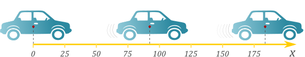
Let’s imagine we record the car’s position along the x-axis every second. If we plot it against time, it would probably look something like the following graph. Keep in mind that the curve is not the car’s trajectory! It merely represents the position of the car along a straight line at any given point of time and can therefore have many shapes, which depend on how the car accelerates.

Every blue dot on our graph represents the position of the car, which is measured on the vertical axis, at the specific second marked on the horizontal axis. Let’s say we want to determine what the car’s average velocity was between the 12th and 36th second after we started measuring time. The car’s initial position at t1=12 s is x1=20 m. At the end of the selected time period, when t2=36 s, the car’s position was x2=160 m.
Using equation 1 we can easily calculate the car’s average velocity within the selected time frame:

If you examine closely, you will notice the car’s average velocity equals the slope, m, of its position vs. time curve, when measured between our two points of interest, namely t1=12 s and t2=36 s.
As discussed above, the resulting value (5,83 m/s) is an average for the selected time slot, which does not mean the car had a constant speed. To verify this, we can calculate the average speed in a shorter time frame, for example, between t1=12 s and t2=24 s. In this case, x1=20 m and x2=65 m, and the average velocity is:

This result implies that, at the beginning, the car was moving slower and then gradually increased its velocity. According to the position vs. time curve, the car’s speed changed even within this new time frame. So, if we take an even smaller one, we might get more information about how the car’s velocity changed second after second. For example, if we calculate de average velocity between t1=12 s and t2=18 s, for which x1=20 m and x2=40 m, we get:

Notice that, as we make the time frame smaller and smaller we approach the car’s speed value at a single instant. This is what we call its instantaneous velocity. Nevertheless, we will never be able to evaluate equation 1 at a single point since a division by zero would be encountered when t1=t2. This is when differential calculus comes in handy.
In order to calculate an object’s instantaneous velocity, we need to make the term t smaller and smaller. A mathematical way to do this is to evaluate the limit of equation 1 when t approaches zero:

We have added a “t” within a parenthesis next to x to remind you that the initial and final positions of a moving body depend on time, furthermore, they are a function of time. Equation 5 is the definition of the derivative of the position with respect to time, which is the proper definition of a body’s instantaneous velocity and can be written as:

Instantaneous velocity is also a vector. Similarly to the average velocity, its direction is that of the object’s displacement vector.
Difference between velocity and speed
We have established that velocity is a vector. This means it has both a magnitude and a direction. Formally, the first one is called the speed of a moving object, and is a scalar value measured in units of length over time, like m/s, km/h, miles/h, etc.
Most of the time we refer to an object’s velocity just by naming the value of length per unit time it travels at. Nevertheless, in those cases we are talking about its speed. It is only when we also mention the direction of movement that we can properly speak about its velocity.
Other helpful sources
Explore this simple but useful simulator by PhET to create the position vs. time plot for a man walking along a straight line at your desired velocity and acceleration. First, click on “charts”, then set up all the variables, and click “play” to create the plot.