
What do egyptian mummies have in common with nuclear plants? At first, you might say: “well, nothing” —but that is definitely not the case! Knowing how to calculate half life will help you discover why:
Most nuclear plants use uranium to generate electricity. This is possible thanks to the fact that this element is radioactive. This means it is unstable and spontaneously emits chunks of its nucleus at very high speeds, which then collide with water molecules causing them to boil. Physicists call this process radioactive decay. Finally, the generated water vapor moves a turbine, producing electricity.
On the other hand, carbon-14 is a type of carbon atom that also exhibits radioactive decay. Living beings like animals, plants, yourself and —at one time— egyptian pharaohs store and renew this element in their bodies while interacting with their surroundings, for example when eating or breathing. Once dead, these organisms cease to ingest carbon-14, and its concentration inside dead tissue starts to decrease due to its radioactive decay.
If you think about it, in both cases the total amount of radioactive substance decreases day by day. Now, how fast does this happen? That is exactly what an element’s half life tells us. Thanks to the fact that we now know how fast most elements decay, we can calculate the amount of radioactive material that remains after a period of time in a nuclear plant or how old an egyptian mummy is based on what is left of it inside its tissues. All of this using the same basic principle: half life.
How to calculate half life
Half life of a radioactive substance is calculated by measuring the time it takes for its activity to decrease by half. A practical way to estimate half life is to measure the activity of the substance as a function of time, plot the results, and perform an exponential fit of the resulting curve. Finally, half life can be extracted from the parameters of the derived equation.
What is half life
Many elements of the periodic table, and specially their isotopes —atoms with the same number of protons as a given element but different number of neutrons—, have unstable nuclei. Such elements are called radioactive. In a spontaneous process called radioactive decay, unstable nuclei emit subatomic particles like protons, neutrons and electrons, or high amounts of energy in the form of gamma rays. This process can initiate a chain reaction, after which atoms with much more stable nuclei are formed.
Radioactive decay is a random process, which means the time needed for an atom to emit radiation is basically uncertain. Just like when flipping coins, you can’t be completely sure about which side they might fall on —even if you know you have a 50/50 chance. All you can do is throw them in the air over and over again until you get the expected result.
Let’s say we do an experiment where thousands of people flip coins and we count those who get tails as time pases. Even though the probability of that happening in each case is 50%, some people might get tails only after several flips, while others might get them right away.
Similarly, a radioactive element has a set probability of undergoing radioactive decay, but we can’t be sure about when it will happen. If we have thousands of atoms of that element, each of them might need a different time to decay. Now, if we were to plot the number of atoms that have not decayed as a function of time, we would get something like this:
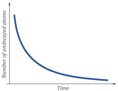
Radioactive decay follows what we call an exponential behavior. This means, the curve above can be described with an equation like this one:
| N=N0e-t | (1) |
In this equation, N is the number of atoms that have not yet decayed; N0 is the original number of atoms when the experiment started; t is time; and is a characteristic value that depends on the specific element under study. Let’s try and understand where this last value comes from.
If we repeat the flipping-coin experiment but this time participants throw dice instead, and we count those who get a 6 as time goes by, we will notice that the resulting curve is a lot less steep than in the first case. This means it takes everybody more time on average to get the desired result. This is simply because throwing a 6 with a die has a lower probability than flipping tails —exactly 16,7% chance.
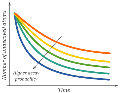
This is again similar to radioactive atoms: different elements have different probabilities of decaying, which implies that their respective “decay curves” will be unique. See the image below: elements with a higher probability of decaying will have steeper curves simply because, in average, they will do so faster. Or, expressed in a different way, the higher the decay probability, the higher the number of atoms that decay per second.
Now, since calculating the probability of the radioactive decay of a certain element might be extremely complex, but measuring time and counting the number of remaining “undecayed” atoms sounds a lot easier, scientists have decided to do the latter. This is where the concept of half life comes from.
Half life, usually denoted as t1/2, is the average time it takes for half of the radioactive atoms in a very large group to decay. The word “average” in this definition refers to the statistical nature of the radioactive decay process. Go ahead and read the section called “Why is half life a statistical value?” to learn more about this through a thought experiment.
As you might have inferred by now, the units of half life are time units (seconds, hours, days, years, etc.). Element’s half lives vary in a huge range: from less than a second to millions of years. See the next table for some examples.
Half lifes of some radioactive isotopes
| Radioactive isotope | Half life |
| hydrogen-7 | 23 x 10-24seconds |
| fluorine-28 | 40 x 10-9 seconds |
| plutonium-228 | 1.1 seconds |
| iodine-131 | 8.02 days |
| carbon-14 | 5730 years |
| uranium-235 | 703.8 million years |
| tellurium-128 | 2.2 x1024 years |
Although usually used to describe the radioactive decay of atoms, half life can also be applied to many other substances which amount or effect decreases with time, for example, chemical compounds inside the human body.
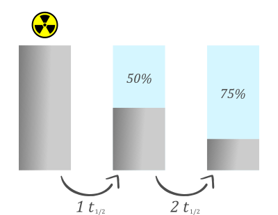
As the following image shows, after one half life, 50% of the original substance is expected to have decayed into its “daughter” substance. Consequently, after a second half life, half of the remaining 50% would have decayed, i.e. 25%, thus leaving a total of 75% of the original amount as daughter substance.
Half life equation
To understand where the half life equation comes from, we need to consider the difference between decayed and undecayed atoms in a very small period of time. We can express this difference mathematically like this:
| dN=Ndt | (2) |
Where, N is the number of atoms which have not decayed, dN the infinitesimal change in the number of atoms that decay, dt the change in time, and the proportionality constant, called decay constant, which is specific to every element.
To understand this equation, just think about the effect of increasing or decreasing every variable. For example, the larger the time is, the larger dN will be, meaning more atoms have decayed. Similarly, the larger the initial amount of radioactive atoms N, the larger the number of those which will decay per unit time, thus the larger dN will be.
The solution to equation 2 above is an exponential function that describes how the number of radioactive atoms pending to decay, (N) changes with time. It also depends on the original number of atoms (N0) and the element-specific decay constant:
| N=N0e-t | (3) |
Half life is defined as the time needed for half of the initial radioactive atoms to decay. Based on the last equation, half life is the value of t for which N=N0/2. If we replace this in equation 3, we obtain:
| N02=N0e-t1/2 | (4) |
Solving this equation for t1/2 yields:
| t1/2=ln(2) | (5) |
This means we can determine an element’s half life by measuring its decay constant from experimental data. The next formula is very intuitive because it relates the final amount of a decaying substance N to its initial amount N0, the substance’s half life t1/2 and the time:
| N=N012t/t1/2 | (6) |
How to find half life
Half life can be measured in laboratory experiments with the use of specialized equipment sensible enough to perceive the particles or gamma rays being emitted by a radioactive sample. The general procedure to determine half life is the following:
- Measure the activity of the radioactive sample under study for a time long enough to notice a significant decrease in counts (this will depend on the element). To complete this step, follow the specific instructions provided by the manufacturer of the sensor you use.
- Perform the measurement again without any sample to determine the background signal. This is the radioactive “noise” that is present in the room you are doing the experiment in and that does not come from your sample.
- Subtract the background signal from the data obtained with the sample.
- Calculate half life life this:
The number of undecayed atoms, N, and the initial number of radioactive atoms, N0, are directly proportional to the sample’s activity A, and its initial activity, A0, respectively. So equation 3 can be converted into this:
| A=A0e-t | (6) |
This is especially useful, since we are not measuring atoms but emission counts. By rearranging and taking the natural logarithm on both sides, equation 6 becomes:
| ln(AA0)= -t | (7) |
If you plot ln(A/A0) vs. time, you should obtain a straight line with a negative slope. That slope is your decay constant! Finally, you can calculate your sample’s half life simply by using equation 5.
Other helpful sources
Many websites offer very helpful tools to calculate and understand half life and radioactive decay. For example, you could use Rad Pro’s calculator to confirm any half life measurement you make. Keep in mind the units used in the app are cpm (counts per minute), which refers to the number of measured emissions from a radioactive atom per minute.
You can also use The Lund/LBNL Nuclear Data Search to find any radioactive isotope by inputting the element’s symbol, atomic number, mass number, or a half life range.
Why is half life a statistical value?
The radioactive decay of atoms is a random process; and half life is related to that. Let’s do a thought experiment to try and understand this:
Imagine you could observe 10 isolated uranium atoms. With time, they would start to decay. In principle, you would expect that after one half life 5 atoms have decayed. Nevertheless, since radioactive decay is completely random, it could happen that all of the 10 original atoms decay suddenly, or that none of them ever do. It could also happen that only 3 atoms decay after one half life, or 7 or any other fraction of the original batch.
In reality, all of these scenarios are possible. So, how can we interpret half life if after one “real” measurement it does not necessarily coincide with the time it takes for half of the initial atoms to decay? The key to understanding this is that whether all scenarios are possible, not all of them are as likely to happen.
If we repeat the exercise of observing 10 isolated uranium atoms several times, and calculate the average time it takes for 5 of them to decay, we would see that this value comes close to the reported half life. In fact, the more we repeat the experiment, the more the average value approaches uranium’s actual half life.