
The confidence interval is an important tool for statisticians and also for the lay people that want to understand to what point they can trust statistical data. For a concrete example, suppose you hear in the news that the State Governor is considered a good administrator by 52% of the population. As you might imagine, not all State citizens were asked their opinion, but only a small fraction of them. How confident could you be that the real majority of the state citizens are by her side? Well, the confidence interval can help you to answer that.
The next day things get even worse: you read about another survey, from a different media outlet, that indicates that only 47% of the population is satisfied with her administration. What now? Is anybody lying? Which pool should you trust more?
There is no way to answer this without knowing the confidence interval of both pools, together with its confidence level. The confidence interval is a range of values which gives a concrete idea of how much the value estimated from a sample can vary if we were to take another sample from the same population.
In the example above, let’s assume that the confidence interval of the first survey is between 49% and 56% and for the second one it is between 46% and 49%. Now it is possible to know that the statisticians of the first pool are not completely sure if the majority of the population is on the Governor’s side, as the mean value of 53% alone would suggest. In fact, their confidence interval says that according to their sample data, it is possible that the real value for the entire population to be 49%.
Meanwhile, the statisticians of the second pool are more confident in stating that the majority of the citizens are not on her side, since the entire interval is below 50%. How sure? That depends on the confidence level.
The confidence interval is closely related to the confidence level and also to the margin of error. It is easy to get confused by them, but after reading this post you will be able to see the differences and relationships among them. Also, you will learn how the confidence intervals can help to achieve a more refined understanding of real-life statistical results.
What is A Confidence Interval
A confidence interval is a range of most probable values for a statistical parameter, under a specified confidence level. The statistical parameter is any information that needs to be computed for a population of any kind.
“Population” in statistics is a set of individual entities that are not necessarily living beings. For example, the population for a statistical analysis could be all the cereal boxes arriving at the end of the assembly line. In such a context, the statistical parameter being measured could be percentual of boxes that are more than 5% below the weight printed in the box.
Usually, weighting every single box coming from a modern assembly line is impractical. A realistic alternative is to analyze a sample of the box population and use the sample to estimate the total number of boxes produced out of the desired standard. The value estimated from the sample is the estimated value.
IMAGE CEREAL BOXES, SAMPLE
The estimated value of a statistical parameter is the most probable value of the “real” population value according to a data sample. However, there is always some probability that the population value is other than the most probable one. Although these alternative values are less probable than the estimated value, they still have a non-zero probability of being the “right” one.
The confidence interval, together with the confidence level
Anyway, when working with samples, there is no guarantee that the population value is indeed inside the confidence interval. The confidence interval is always related to a specific confidence level. The most common confidence levels used for statistical calculations are 90%, 95% and 99%.
It is important to understand exactly what those numbers mean. A 95% confidence level states that if new samples would be collected several times from the same population, in 19 out of 20 samples, the estimated value would be within the confidence interval.
Why confidence interval is important
Suppose the town police need to know how many people are going to the 4th of July parade, so that they can prepare safety measures. The town’s statisticians perform a survey and tell the police that the estimated value is 24,750 people with a 95% confidence level. The new Sheriff does not know about confidence levels, but 95% doesn’t sound as a good enough confidence for him. Then, he demands a 99% confidence level.
The statisticians get angry, and instead of gathering a larger sample, they decide to just recalculate the numbers with the desired confidence level. The new report offers what the Sheriff asked for: now the statisticians are 99% sure the number of people attending the parade will be somewhere between 500 to 50,000. This is the new confidence interval needed for achieving a 99% confidence level from that sample.
Of course, such a large range of possibilities is not very useful. After all, taking care of 500 happy folks is an entirely different task than controlling a mob of 50,000 people.
The Confidence Interval Formula
Most statistical calculations assume a random statistical parameter, which means that the parameter values follow the normal distribution, also known as the bell curve. In most cases, this is a good enough approximation to reality. Then, the confidence interval is the range of values that need to be taken into account in the bell curve to achieve the established confidence level. This value also happens to be the area under the selected portion of the curve.
Figure xx illustrates these concepts. It is possible to see that the higher the demanded confidence level, the larger the confidence interval (for the same sample). However, as you have seen in the police example, if the confidence interval is too large, the statistics can turn out useless in the real world.
IMAGE
The confidence interval formula is this:
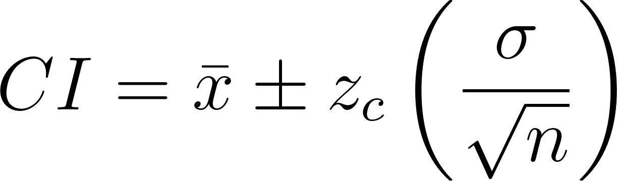
Where:
- is the mean value for the statistical parameter;
- is the standard deviation;
- is the sample size
- is a tabulated value dependent on the confidence level, that adjusts the data for the normal distribution.
The formula represents an interval equally distributed () around the mean. The value added in each side of the mean is known as the margin of error
We can see from the formula that the width of the interval depends on the variation of values inside the sample. In addition, a larger sample reduces the confidence interval, making the estimated value more precise.
However, the square root on n indicates that the effect of increasing the sample size of smaller samples is stronger than for larger samples. In other words, increasing the sample size from 20 to 50 is more effective than increasing the sample size from 100 to 130, although the absolute increase in both cases is 30 individuals. In real life, this means that there is a practical limit where increasing the sample won’t be worth the tiny reduction in the confidence interval.
Finally, there is a subtle issue with the formula above. The problem is that it depends on the population standard deviation (σ). But because we are dealing with samples, the population standard deviation is unknown. For large samples, it is possible to trust that the estimated value S is close enough to the population value σ.
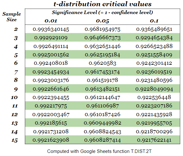
In contrast, for small samples the best confidence interval formula is one that adjusts for the student distribution instead of the normal distribution. In this case, the formula is almost the same, but is substituted by for the t-distribution and the standard deviation is substituted by the estimated standard variation S:

How To Find Confidence Interval
From the formula you know that the size of the confidence interval depends on how much variation there is in the population for that statistical parameter. And the variation is intrinsic to the population composition. For example, to estimate the average age of all people attending college in the US, one can expect a relatively low variation. However, if the goal is to estimate the average age of all people in a town with a similar population size, the variation can be expected to be much higher.
The sample size also interferes with the width of the confidence interval, since smaller samples have a higher risk of not reflecting the real population composition.
Meanwhile, to get (or , for small samples) one usually consults a table of pre calculated values or uses some statistical application. A small t-distribution table can be seen below.
.

Now we can calculate the confidence interval of a small sample. Suppose the values below are ages from random US college students.
Thus, we need the average age and the standard deviation for this sample. In the table there are also the values of the squared deviation from average value, that will allow us to calculate the variance, thus the standard deviation.
Using the values from the t-distribution table for a sample size of 12, we can then compute the confidence interval at a 95% confidence level.


Using these values, the confidence interval is calculated like this:
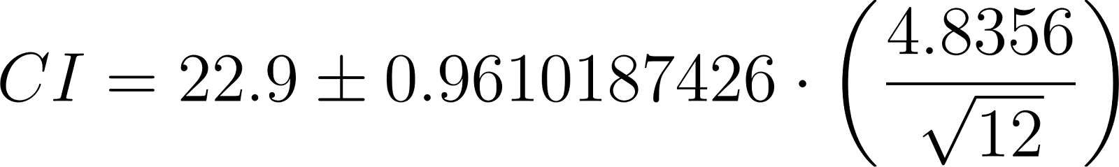
With the final result being:

It is important to know how to interpret this result. It means that if we were to collect new samples from the population of US college students, 19 out of 20 times their average age would be between 21.6 and 24.3 years.
You can try to calculate the confidence intervals at 90% and 99% confidence levels as an exercise. You’ll see that the values will change only slightly, since the ages of this population vary way less than the overall population ages.
Confidence Interval and Statistical samples
Ideally, one would include the entire population in the statistical computation to obtain the exact numbers. Unfortunately, this is only feasible in a few real-world scenarios. For example, any company could easily compute the exact value of the average time their employees in leadership positions stay in the job. Similarly, a robotics Professor can know exactly which of his students have grades within the highest 25% of all grades in the class. Then he can select only among them for creating a competition team.
In most real-life cases, though, gathering the data from the entire population is too expensive or even impossible. For those situations, statisticians estimate the population value by computing them for smaller samples of that population. In this case, their calculations provide what is known as estimated value. The “thing” that is being estimated from the sample is known as the statistical parameter. In our first example, the statistical parameter is the percentage of citizens who are satisfied with the Governor’s administrative skills. In the 4th of July example, the statistical parameter is the number of people that will attend the event.
Sampling Methods and Confidence Level
There are many sampling methods out there that try to provide the researcher with samples that are representative of the population. In other words, the most appropriate sampling method will generate a sample whose composition is similar to the population’s composition. In the pool about the Governor’s popularity, this would mean that if 52% of the state population is female, the sample should reflect this. If 10% of the citizens are unemployed, 10% of the sample should be searching for a job too.
Choosing the factors that will be considered to understand the population’s composition is a mix of science and art. No sampling method guarantees samples with the exact same composition as the population’s. That’s why we need to define the acceptable confidence level for the estimated value.
Confidence level and Confidence Interval
By using samples to represent an entire population, you automatically admit that you are going to deal with uncertainty. Usually, the “acceptable” uncertainty level is decided in advance by choosing the confidence level before sampling. The confidence level helps to define a sample size which will (hopefully) be able to produce a confidence interval that is useful enough for the application.
It is quite intuitive that larger samples lead to estimated values that are closer to the population value. However, in real life statistics, larger samples also mean more resources: more people, more money, more computational power and more time to get to the results. Thus, the choice of the confidence level – and therefore the confidence interval obtained – reflects a balance between accuracy and cost.
